Overview
The Capacitated Vehicle Routing Problem (Cvrp) is an optimization problem that consists of charting optimal routes to deliver goods to a given set of customers using a fleet of vehicles with capacity constraints. The objective of the Cvrp is to minimize the total distance, or “cost”, of all of the routes.
The motivations here are clear: minimizing the driving distance of your delivery fleet minimizes fueling costs, and thus produces greater profits overall. The challenges are abound though: Cvrp is \(\textsf{NP}\)-hard, and so developing a deterministic algorithm that produces optimal results while still operating under reasonable computation bounds is difficult and unpractical.
In Spring 2019, Andrew Wagner and I took on the challenge of developing a local-search-based solver for a set of Cvrp instances. With some carefully crafted metaheuristics, some engineering optimizations, and a little bit of luck, our Python solver (at a concise ˜200 lines of effective code!) produced the most optimal results when compared against 21 other implementations on 16 large-scale instances of the problem. Specifically, our solver:
-
Produced the most optimal solutions on 6 of the 16 instances (with the next highest teams producing 5, 2, and 2 most optimal solutions).
-
Placed in the top three of all teams over all instances when evaluated on solution optimality, with an average rank of 1.8 (out of 21, where 1 is the best) over all instances.
The Problem
Each Cvrp instance consists of three parameters: \(num\_vehicles\), or the number of vehicles that are available in the fleet; \(vehicle\_capacity\), the amount of units each vehicle can hold; and a finite set of \((demand_i, x_i, y_i)\) tuples for \(1 \leq i \leq n\), where each tuple represents a customer’s location and the number of units that needs to be delivered to them.
$$ \begin{align*} instance \thinspace := \enspace ( & num\_vehicles, \\ & vehicle\_capacity, \\ & \{ (demand_1, x_1, y_1), ..., (demand_{n}, x_{n}, y_{n}) \}) \\ \\ \mathrm{where} \quad & num\_vehicles \in \mathbb{Z}_{>0} \\ & vehicle\_capacity \in \mathbb{R}_{>0} \\ & (demand_i, x_i, y_i) \in (\mathbb{R}_{\geq 0} \times \mathbb{R} \times \mathbb{R}) \quad \mathrm{for} \enspace 1 \leq i \leq n \end{align*} $$
A solution to a Cvrp instance is a set of variable-length tuples which each denote the route of a particular truck. The set has cardinality \(num\_vehicles\) such that each vehicle in the fleet is given a route. (We’ll denote when a vehicle is routed to a given customer \(i\) by their \(i\) index in the set of \((demand_i, x_i, y_i)\) tuples.)
$$ \begin{align*} solution \thinspace := \enspace & \{ route_0, ..., route_{(num\_vehicles - 1)} \} \\ \\ \mathrm{where} \quad & route_i \subset \mathbb{Z}_{\geq 0} \qquad \mathrm{for} \enspace 0 \leq i \leq num\_vehicles - 1 \\ & |route_i| \neq \infty \,\qquad \mathrm{for} \enspace 0 \leq i \leq num\_vehicles - 1 \end{align*} $$
Each instance implicitly defines a set of constraints on the set of valid solutions:
- Maximum Trucks: The number of trucks we can utilize is equal to \(num\_vehicles\).
- Maximum Capacity: Each truck can only deliver up to \(vehicle\_capacity\) demand.
- Trucks Return Home: Every route needs to start and end at the delivery hub (denoted by the “customer” with index \(0\)).
Given this specification, the challenge is to produce an optimal solution, where “optimal” is defined as the solution that satisfies all of the constraints of the problem while minimizing the total distance travelled by all vehicles on their routes.
$$ \begin{align*} \mathrm{minimize} \quad \sum_{i = 0}^{num\_vehicles - 1} \sum_{j = 0}^{|route_i| - 1} \mathrm{dist}(route_i[j], route_i[j + 1]) \end{align*} $$
In this variant of Cvrp, we’ll make two simplifying assumptions:
- Visits Fully Satisfy: When a truck visits a customer, it must satisfy all of the customer’s demand at once. In other words, a truck will not make a “partial delivery”. This means that a customer should never be visited twice.
- Trucks Travel Once: When a truck leaves the hub and eventually returns back to the hub, it will not depart the hub again. Thus, a vehicle’s capacity is exactly the amount of capacity they can handle when deliveries happen (i.e. it cannot return back to the hub to pick up more demand).
With the specification in mind, we set out to develop a solver that would generate solutions for Cvrp instances.
The Solver: Local Search
Our local search routine was inspired by the local search framework from Paul Valiant’s CSCI1570. The intuition behind this framework is that we can use a standard framework that allows us to move through the solution space iteratively by starting from one solution and moving to a “nearby” solution via problem-specific proposal functions. We can then determine the usefulness of a newly found solution using a problem-specific objective function. Proposals and objectives are then tied together with the following two additional components:
-
The acceptance criterion, which determines if we accept a given proposal solution (and thus start the next loop iteration with our newly proposed solution), or reject the solution and retry again with our previous solution.
To determine if a solution is acceptable in the search, we then use an acceptance epsilon which sets the threshold at which we will allow searches to perform worse with the expectation that they will allow us to escape local minima. This is a reflection of the “exploration-vs-exploitation” tradeoff problem in local search algorithms—while we want to exploit the regions of the solution space which seem to be promising, we also want to make sure we explore other regions since we only have local knowledge of where we are in the solution space. Thus, if we don’t explore enough, we might get stuck in a convex region of the function while attempting to exploit a local minima of the function, even though this area will not lead to its true minimum.
-
The stopping condition, which determines when we stop the local search routine. The basic stopping condition is an improvement timeout—that is, if you don’t see enough improvement within a certain time delta, then the local search should terminate.
Our solver uses a somewhat more complicated approach to deciding on a stopping condition, though this approach is meta to the actual local search process and thus is not important directly to the implementation of a local search routine. (This approach is described in the “Simulated Annealing” section below.)
How the proposal functions and objective function are used within the local search framework does not generally change from problem-to-problem. We can thus separate our concerns and utilize a problem-agnostic framework that helps constrain our work to designing effective heuristics for the proposal function which makes for easier testing and design.
To do this, we implemented a local_search routine with the following signature (where Solution is some arbitrary interface):
def local_search(objective_function: Callable[[Solution], Number],
                 proposal_function:  Callable[[Solution], Solution],
                 initial_solution:   Solution,
                 acceptance_epsilon: Number,
                 improvement_time:   Number,
                 improvement_delta:  Number) -> Solution:
    """
    General-purpose local search minimization function.

    @param objective_function: The function to minimize.
    @param proposal_function: The function that gives us new solutions.
    @param initial_solution: The initial Solution to start minimizing
        from.
    @param acceptance_epsilon: A value for promoting exploration vs
        exploitation. New Solutions are accepted if they improve the
        objective function's value, or if they do not make it worse
        than the value of this parameter.
    @param improvement_time: The amount of time (in seconds) we're
        willing to wait before we see a "significant" improvement,
        where the "significance" of a Solution's contribution to the
        objective function is defined by improvement_delta.
    @param improvement_delta: The minimum amount of improvement that
        needs to happen in a given time period of improvement_time
        before we terminate.
    """
    ...
local_search itself is implemented as a simple loop with some conditionals:
-
Pass the
Solutionfrom the previous iteration into theproposal_functionto generate a candidateSolution. -
Apply the
objective_functionto the candidateSolution. -
If the candidate
Solution’s objective value is better than the current solution’s objective value or is withinacceptance_epsilonunits of the current objective value, update the currentSolution. -
If the candidate
Solution’s objective value is better than the best objective value we’ve seen so far, update the best objective value we’ve seen so far. -
If the current
Solutionhasn’t been changed in the lastimprovement_timeseconds, terminate and return the currentSolution.
    \begin{algorithm}
    \caption{Problem-agnostic local search}
    \begin{algorithmic}
      \INPUT ($\Theta$, $\rho$, $solution$, $\epsilon$, $\tau$, $\Delta$), where $\Theta$ is objective function; $\rho$ is proposal function
      \OUTPUT best solution found during local search
      \ENSURE objective value of output $\leq$ objective value of $solution$
      \STATE $\delta_\text{goal} \gets \Theta(solution) - \Delta$ \COMMENT{improvement needed before timeout ($\tau$)}
      \STATE $best \gets solution$
      \WHILE{time since $\delta_\text{goal}$ last updated $< \tau$}
        \STATE $candidate \gets \rho(solution)$
        \IF{$\Theta(candidate) < \Theta(solution) + \epsilon$}
          \STATE $solution \gets candidate$ \COMMENT{$candidate$ accepted}
          \IF{$\Theta(solution) < \Theta(best)$}
            \STATE $best \gets solution$
            \IF{$\Theta(best) \leq \delta_\text{goal}$}
              \STATE $\delta_\text{goal} \gets \Theta(best) - \Delta$ \COMMENT{reset improvement goal and reset timeout}
            \ENDIF
          \ENDIF
        \ENDIF
      \ENDWHILE
      \RETURN $best$
    \end{algorithmic}
    \end{algorithm}
With local_search implemented, the main work involved is in figuring out how to best apply such a routine to Cvrp. We discuss our Cvrp-specific work below in four parts.
Heuristics
Our first goal was to determine what a Cvrp proposal_function should look like. One approach for formulating proposal functions is to try to analyze various facets about the problem and then come up with a single overall proposal. However, a key insight is that instead of trying to form one optimal kind of proposal, we can simply come up with multiple proposals and choose randomly among them each time we need to look at a solution. While this might seem wasteful (especially if one just adds a proposal function that isn’t particularly effective), the intuition behind why this approach is still effective is that adding “too many” proposal functions will only decrease our performance by a constant while missing a critical proposal function might prevent us from moving past a blocking frontier in the solution space.
In the end, we created five proposal functions that aimed to express various intuitions we had about the shape of the problem space. We describe these metaheuristics in detail below, but one thing worth noting that might seem to contradict the previous paragraph is that we found that some proposal functions were effective very early on in the local search process and then became extremely ineffective as the function converged towards its true minimum. We thus applied our local_search routine in such a way that allowed us to remove some proposal functions after some amount of time had passed during the search.
Recall that our solution space consists of multiple sets of vehicle routes of various lengths. Our metaheuristics can thus be divided into two categories: proposals that make changes within one specific route, and proposals that make changes across two routes.
Within Routes
These proposal functions focus on making local moves within one specific route. (They’re implemented simply by randomly picking one of the routes in the current Solution and then applying the described move to that route.) Since optimizing for the minimum distance within one specific route effectively reduces to the Traveling Salesman Problem (Tsp), both proposals are taken directly from the standard handbook of Tsp local search metaheuristics.
-
2-opt: This heuristic implements the 2-opt swap for Tsp, with the goal being to find routes that cross over themselves (or, more generally, perform some degree of backtracking) and reorder its nodes in such a way that it does not.
Literature for the Tsp generally describes this move as picking two random edges in the route, deleting them, and then reconnecting the resulting subgraphs in a different way. I think a more intuitive way to think about this move is that it selects a random, variable-length segment of nodes and reverses the order of the segment in the route (as illustrated in the diagram shown here).
![]()
Visualization of a 2-opt swap. -
3-opt: This heuristic implements the 3-opt swap for Tsp. This involves picking three random edges in the route and then trying to reconnect each of the resulting subgraphs. The reconnected route with the most optimal objective value (i.e. the lowest value) is then returned from the proposal function.
3-opt is more complicated and takes more time than 2-opt, and there exist sequences of 2-opt swaps that would effectively result in the same route that a 3-opt swap would produce. However, such a sequence might include prerequisite moves that increase the length of the route which may result in the acceptance criterion of the local search algorithm rejecting those sequences and preventing further exploration.
![]()
Visualization of a 3-opt swap.


More complicated Tsp heuristics were considered for proposal functions. However, given that vehicles have a limited capacity in Cvrp, routes are small and the optimization combinatorics within routes were small as well. Thus, the solver was generally able to ensure that each route visited its assigned locations in the shortest way possible.
Across Routes
These proposal functions focus on making local moves across two routes. (They’re implemented simply by randomly picking two of the routes in the current Solution and then applying the described move to that pair of routes.)
-
Relocate: This heuristic moves a customer from one route to another route. It does this by randomly picking a customer in one of the routes, and then moving that customer to a random location in the other route.
![]()
Visualization of the "Relocate" move. -
Swap: This heuristic swaps a pair of customers in each route to another route. It does this by randomly picking a customer in each route and then swapping them in their respective routes.
A potentially more effective variant of the swap heuristic would be to swap entire segments between routes (similar to how the 2-opt Tsp heuristic works), though this was not explored in-depth in our implementation.
![]()
Visualization of the "Swap" move. -
Cross: This heuristic aims to remove unnecessary overlaps between routes by swapping the end segment of one route (where the “end segment” is randomly picked within the proposal function) with the end segment of another route (the “end segment” here is chosen randomly as well).
![]()
Visualization of the "Cross" move.


All of these proposal functions are stochastic and purely local. They make no reference to the actual spatial properties of each of the customers in the Cvrp instance, and thus each across-route proposal function needs no understanding of the actual instance in order to effectively make optimal moves. While this may make the effectiveness of these proposal functions seem surprising, we believe that the low computational overhead for each of these proposals allows them to be invoked more frequently. Thus, more potentially optimal moves are explored during the local search, in comparison to a more “clever” approach which might miss surprisingly effective moves in the process.
Simulated Annealing
Since the solution space for Cvrp consists of discrete elements, local moves can generally produce large improvements at first but result in diminishing returns later on. These diminishing returns can be a result of getting stuck in a local minima; conversely, they can be a result of not focusing enough on exploiting a decreasing region and making too many moves around the solution space.
To mitigate these concerns, we used a technique known as simulated annealing. At a high level, the simulated annealing metaheuristic invokes the local_search procedure as described above, but dynamically adjusts the acceptance criterion instead of leaving it at a constant value. The criterion initially starts out flexible, resulting in the acceptance of many local moves even if they worsen the optimum value by a reasonably large value. This allows the solver to perform a more extensive search on interesting regions of the search space and prevent it from getting stuck in local minima early on. As time goes on, we tighten the criterion—the tolerance for bad moves is lowered and more moves are rejected, allowing the solver to focus on exploiting decreasing regions of the objective function.
In our specific local_search function, the acceptance_epsilon, improvement_delta, and improvement_time parameters allow us to easily customize our exploration tolerance whenever we make a call to the function. With some trial-and-error and some best-guesses, we found that the following annealing schedule was effective for our class of Cvrp instances:
epsilon_schedule     = [1000, 100, 50, 10, 5,  2,  1.5, 1,  0.5, 0.1]
improvement_schedule = [100,  10,  8,  8,  7,  6,  3,   3,  1,   0.5]
timeout_schedule     = [2,    4,   6,  12, 8,  8,  6,   5,  4,   4]
These hyperparameters were chosen by hand and with trial-and-error, though interestingly we found that at least our epsilon_schedule follows a somewhat logarithmic pattern.

Our solver needed to handle both large instances and small instances, which explains the wide range of epsilon values displayed in the annealing schedule were motivated by our solver’s need to handle both large-scale instances (for example, with all locations fitting inside of a 4000 unit square) and small-scale instances (with locations fitting under 100 units, etc.). However, some of the small instances had objective values of less than 1000 on their base initial solution alone, which made some of the early phases of the annealing schedule particularly ineffective.
To combat this, we had our solver skip certain calls to local_search early in the schedule if the epsilon was less than one-third of the initial solution’s objective value. This “one-third” value was chosen arbitrarily and after some trial-and-error on our test data, but we found that it was particularly effective on small instances at cutting out early phases that would ultimately just make no progress and waste time waiting to time out (according to the timeout_schedule).
    \begin{algorithm}
    \caption{Simulated annealing technique}
    \begin{algorithmic}
      \REQUIRE lengths of $epsilon\_schedule$, $timeout\_schedule$, and $improvement\_schedule$ are equal and non-zero
      \ENSURE objective value of $solution$ is non-increasing after each iteration
      \STATE $solution \gets$ initial solution
      \STATE $initial\_objective \gets $ \texttt{objective\_function}($solution$)
      \FOR{$i \gets 0$ \TO length of $epsilon\_schedule - 1$}
        \STATE $\epsilon \gets epsilon\_schedule[i]$
        \STATE $\tau \gets timeout\_schedule[i]$
        \STATE $\Delta \gets improvement\_schedule[i]$

        \IF{one-third of $initial\_objective \geq \epsilon$} \COMMENT{skip large phases}
          \STATE $solution \gets$ \texttt{local\_search}(\texttt{objective\_function}, \texttt{proposal\_function}, $solution$, $\epsilon$, $\tau$, $\Delta$)
        \ENDIF
      \ENDFOR
    \end{algorithmic}
    \end{algorithm}
An alternative approach we considered to mitigate the “large vs small instance epsilon” calibration issues was to use percentage-based epsilons, where the epsilon would be some decreasing percentage of the current objective value. While this seemed cleaner to implement compared to the “one-third” skip trick mentioned in the previous paragraph, we found that this caused the local search to get stuck too quickly on small instances because of the discrete nature of the problem. It was difficult to calibrate exactly what kinds of percentage epsilons would work on both small-scale and large-scale instances, and thus we found that just using the integer-based approach worked better with the solution space at play.
Feasibility
One issue that our solver needs to deal with is ensuring that it restricts itself to valid candidates in the solution space. The high-dimensionality and constraints of Cvrp make it difficult to find an initially valid solution to begin with!
We implemented two techniques in our solver to help with the process of reaching the valid region of the solution space while still allowing us to take advantage of the performance benefits of local search.
Ghost Vehicles
While each Cvrp instance only provides for \(num\_vehicles\) vehicles in a valid solution, we initialized our solutions to contain \(num\_vehicles + 1\) routes. This extra “ghost vehicle” holds unassigned customers and acts as a temporary container until a customer has been assigned to a valid route.
If any customers are currently being served by the “ghost” vehicle, the distance traversed by the “ghost” vehicle is multiplied by a large constant as a penalty within the objective function. (We arbitrarily decided on 100000 as our constant based on the scope of the instances we were tasked with solving.) This incentivizes the local search algorithm to move as many things out of the “ghost” vehicle as possible as to lower the objective function’s value.
Multiplying the ghost vehicle’s distance by a constant is preferable to simply returning \(\infty\) (as what our objective function would do if any of the capacity constraints were violated by a route) for two reasons:
-
It allows our objective function to “express” how close it is to the valid region of the solution space. If \(\infty\) was returned when any customers were served by the ghost vehicle, regardless of how many customers needed to be moved (all customers vs just one customer), the objective function would not express that the solution had improved in any way. Then, getting stuck in the invalid solution region was easier since no distinction between invalid solutions (since they would all have objective values of \(\infty\)) makes it easy to backtrack farther away from the valid solution region (for example, by moving vehicles out of valid routes back into the ghost vehicle).
-
Improvements in route distance are captured by the objective function even if elements still remain in the ghost vehicle, whether in routes that represent actual vehicles as well as routes within the ghost vehicle. This allows improvements towards the true optimum to be made even if the ghost vehicle has not yet been fully resolved, and essentially allows
local_searchto multipurpose the computation time spent on resolving the ghost vehicle for improving overall routing distance on the valid portions of the solution.
Greedy Binpacking
Throughout most of the development process, we started with setting our initial local search solution to a solution where all other vehicle routes were blank and the ghost vehicle contained all possible customers. However, we noticed that this would waste time early in the local search process as the solver attempted to find the valid region of the solution space.
To expedite this process, we initialized our initial solution using a first-fit descending greedy bin packing algorithm. The algorithm performs an in-order traversal over all \((demand_i, x_i, y_i)\) tuples (each representing one customer that needs deliveries) and attempts to assign them to the first vehicle with remaining capacity. If no route remains that will accomodate a given customer, the algorithm assigns the customer to the ghost vehicle.
    \begin{algorithm}
    \caption{Create initial solution from \textsc{Cvrp} instance}
    \begin{algorithmic}
      \INPUT $(num\_vehicles, vehicle\_capacity, \{(demand_i, x_i, y_i), ...\})$
      \OUTPUT initial solution to be passed to \texttt{local\_search}
      \STATE $routes \gets [\{\}~\textbf{for}~0 \leq i < num\_vehicle]$ \COMMENT{track customers assigned per vehicle}
      \STATE $ghost \gets \{\}$
      \FORALL{$(demand_i, x_i, y_i)$ in demand-descending order}
        \STATE $assigned \gets$ \FALSE \COMMENT{used for ghost vehicle assignment}
        \FOR{$v \gets 0$ \TO $num\_vehicles$ \AND \NOT $assigned$}
          \IF{$\left ( \sum_{j \in routes[v]} demand_j \right ) + demand_i \leq vehicle\_capacity$}
            \STATE $routes[v] \gets routes[v] \cup \{i\}$
            \STATE $assigned \gets$ \TRUE
          \ENDIF
        \ENDFOR
        \IF{\NOT $assigned$} \COMMENT{customer did not fit in any route}
          \STATE $ghost \gets ghost \cup \{i\}$
        \ENDIF
      \ENDFOR
      \RETURN $(routes, ghost)$
    \end{algorithmic}
    \end{algorithm}
This allowed us to place most, if not all, of the customers for a given Cvrp instance immediately so the solver no longer had to worry about finding feasible solutions and could focus on finding more optimal solutions.
Results
Our solver performed the best compared against 21 other implementations submitted by other teams enrolled in CSCI2951O. Solvers were evaluated against 16 instances of varying scope with a solving time limit of 300 seconds, with the largest instance going up to 386 customers and 47 vehicles.
Some statistics on our solver’s performance:
-
Produced valid solutions under 194 seconds on all instances.
-
Produced the most optimal solutions on 6 of the 16 instances (with the next highest teams producing 5, 2, and 2 most optimal solutions).
-
Placed in the top three of all teams over all instances when evaluated on solution optimality, with an average rank of 1.8 (out of 21, where 1 is the best) over all instances.
Final Presentations
Some photos from the final presentation day showcasing class-wide comparisons and results:


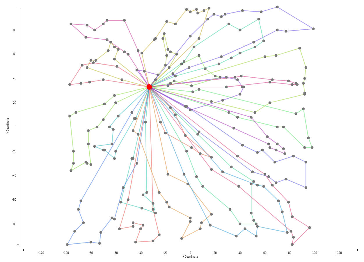
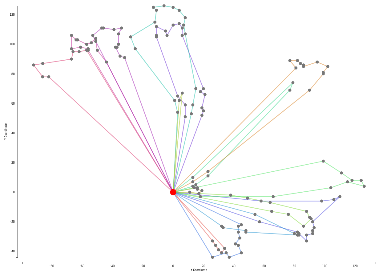
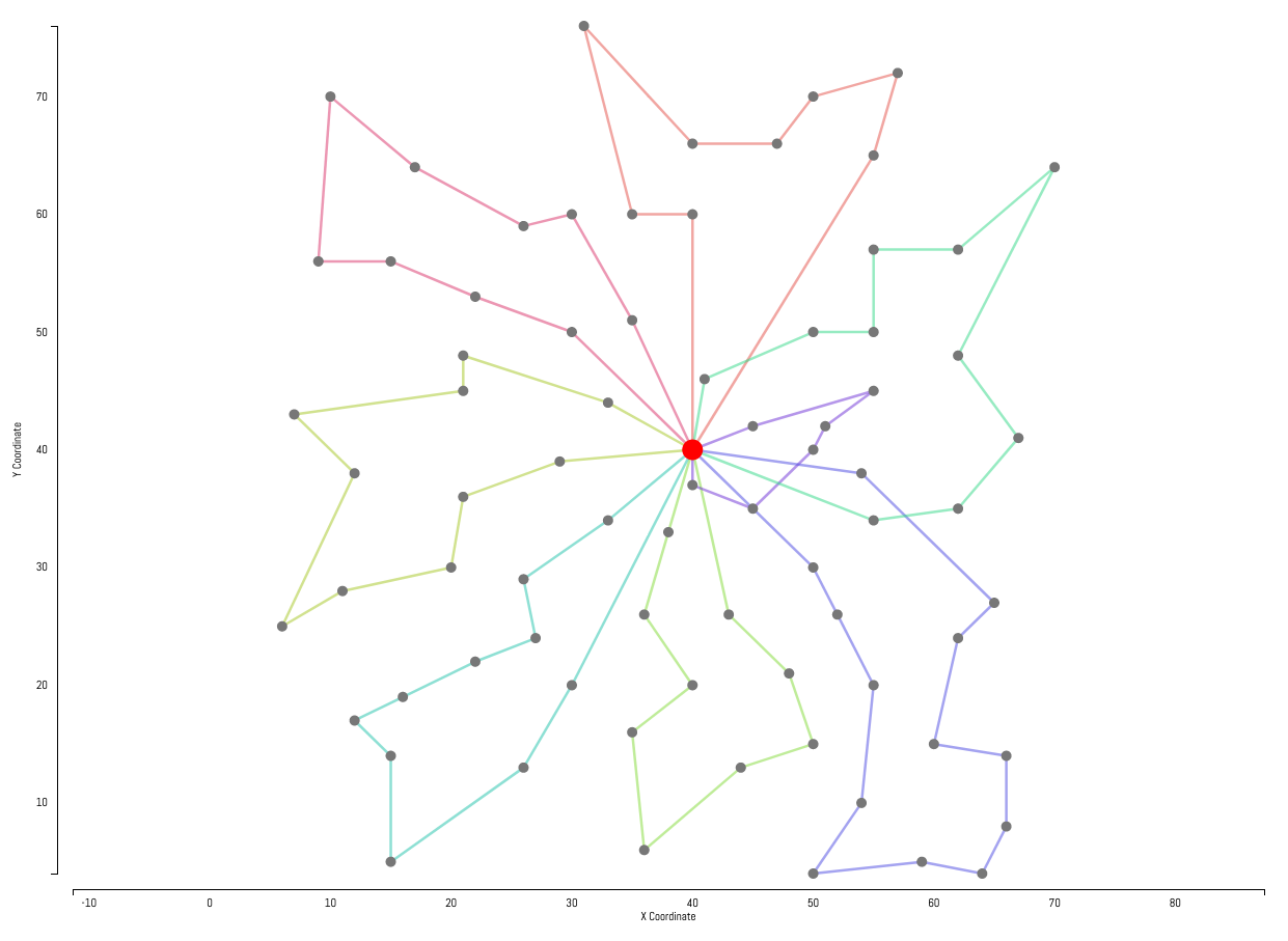
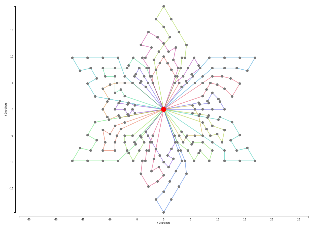
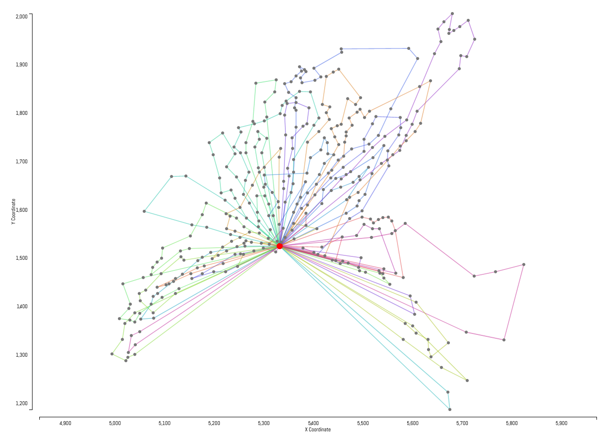
Examples
Example solutions produced by our solver are displayed below. Customers are represented by gray dots with the central hub represented by the larger red dot in the center of each instance. Each customer has a hidden demand not shown in the instance visualizations. Individual routes generated by the solver are represented by the colored lines.